Manifold Sculpting

What Is a Manifold?

High-dimensional datasets often live on a lower-dimensional surface — a manifold — that is crumpled up inside the ambient space. A classic toy example is the Swiss Roll: a 2-D sheet rolled into 3-D. Linear methods like PCA see only the 3-D spread and cannot recover the flat sheet underneath. Nonlinear techniques like Manifold Sculpting can.

What the Algorithm Preserves: δ and θ

Manifold Sculpting anchors its fidelity on two local geometric quantities measured for every point and each of its k-nearest neighbors:

δ_ij — the Euclidean distance from point p_i to its neighbor n_ij, and θ_ij — the angle at n_ij between p_i and the most-collinear neighbor m_ij.

Left: distances δ from a point to its neighbors. Right: angles θ measured at each neighbor.

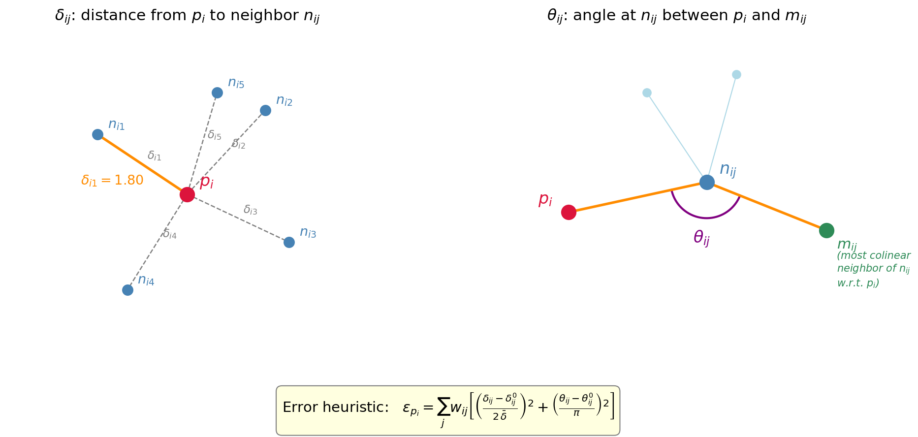
Together, these two quantities capture both the scale (how far apart are neighbors?) and the shape (what direction are they in?) of the local neighborhood. The algorithm's error heuristic penalizes deviations in both:

The Sculpting Process

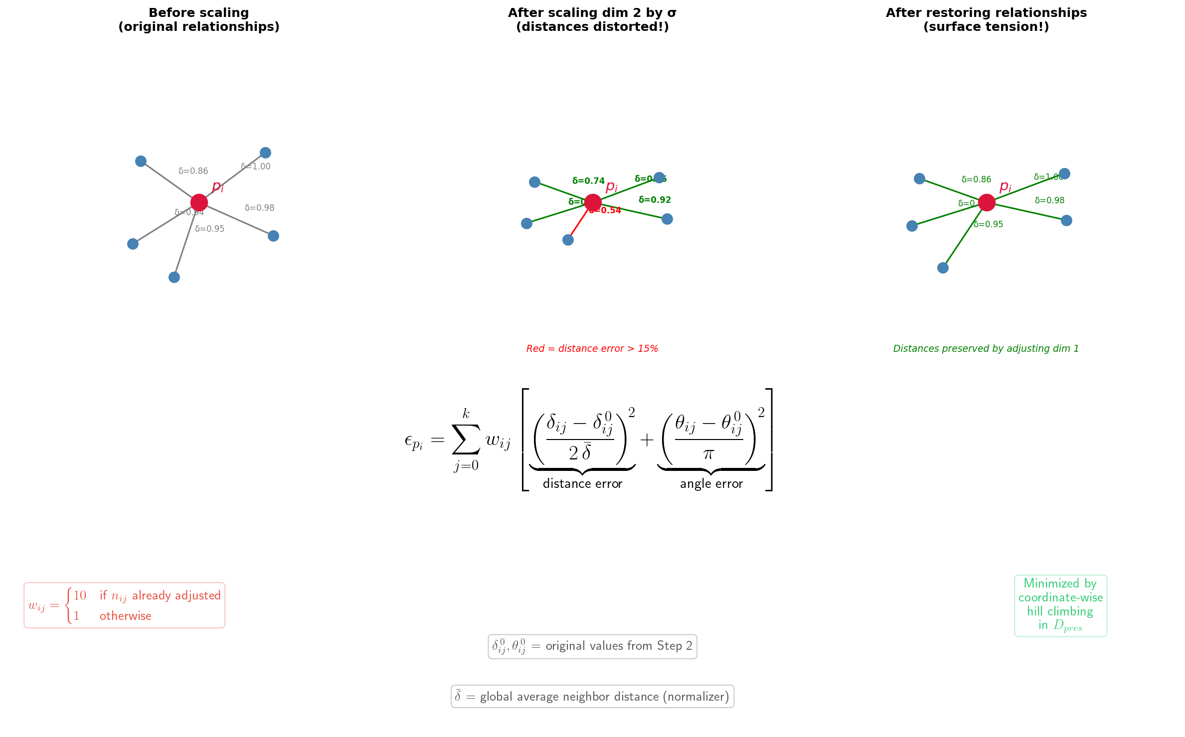
Sculpting proceeds iteratively. At each step, the dimensions targeted for removal are scaled down by a factor σ (e.g. 0.99), which distorts local neighborhoods. The algorithm then traverses every point via breadth-first search and nudges it to restore the original δ and θ values — like a surface under tension snapping back into shape.

After enough iterations the unwanted dimensions are effectively zero and can be dropped, yielding the final low-dimensional embedding.

How Does It Compare?

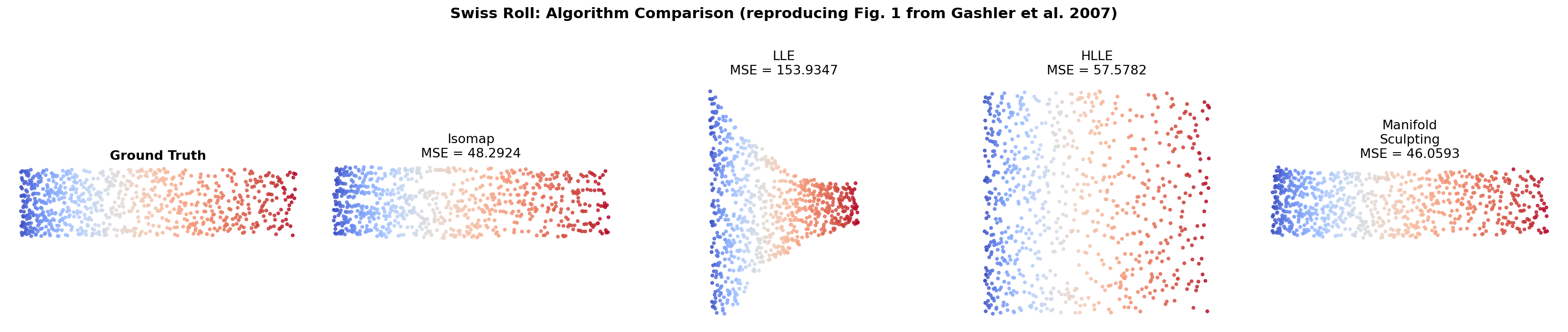
The chart below reproduces the Swiss Roll benchmark from the original paper. Each panel shows the 2-D embedding produced by a different algorithm, colored by the ground-truth parameter. A perfect result would recover the original rectangular color gradient with no folds or tears.

Ground truth vs. Isomap, LLE, Hessian LLE, and Manifold Sculpting. Mean Squared Error (MSE) is shown for each method.

Beyond the Swiss Roll: S-Curve

To confirm the algorithm is not over-tuned to a single manifold, here it is applied to an S-Curve — a surface with non-uniform curvature. The sculpting process cleanly flattens it into 2-D while preserving local neighborhoods.

The Five Steps

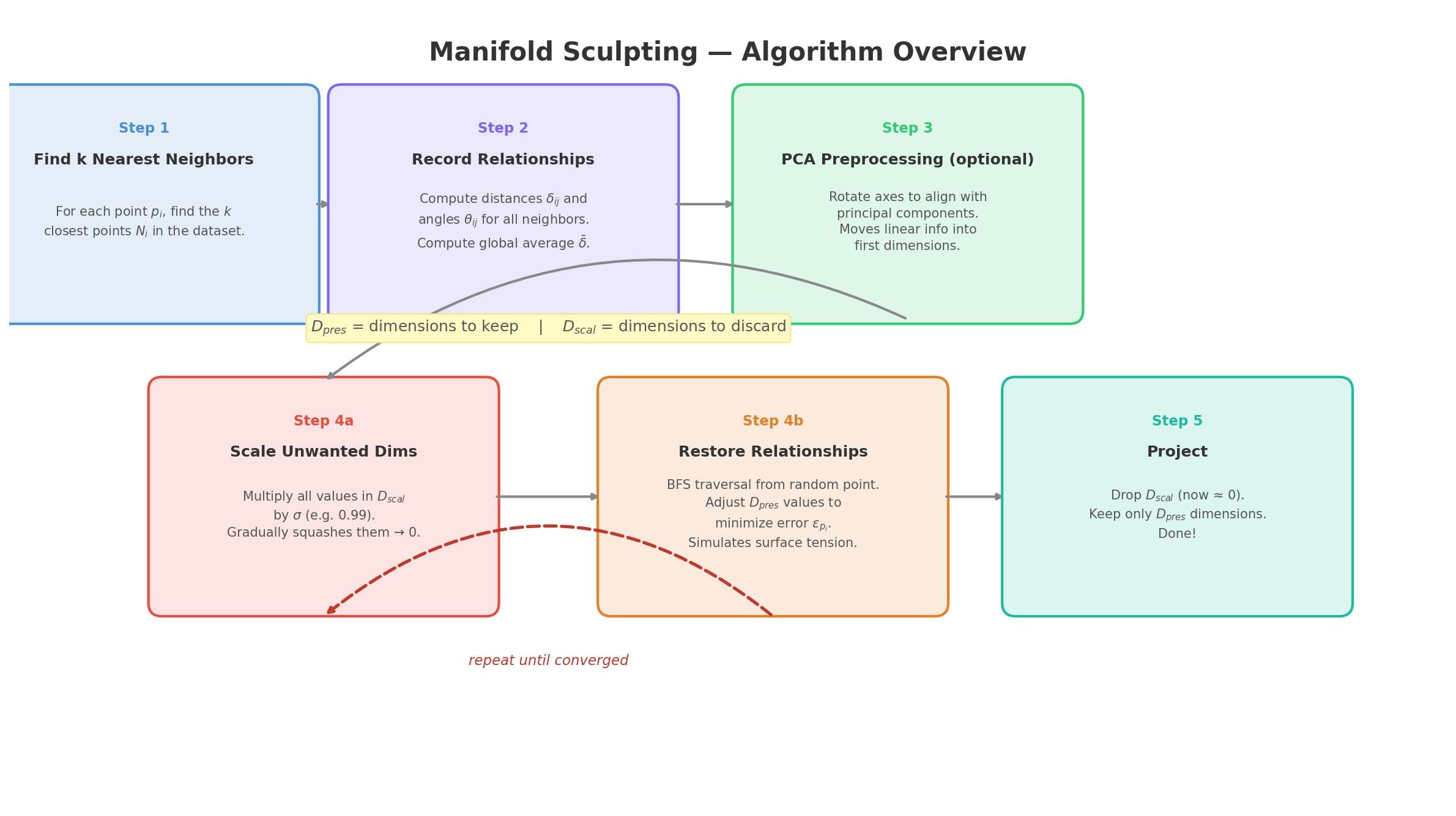
At a high level, Manifold Sculpting consists of five stages:

1. Compute k-nearest neighbors for every point.
2. Record initial δ and θ values; compute the global mean distance δ̄.
3. (Optional) Pre-process with PCA so the first axes carry the most variance.
4. Iterate: scale unwanted dimensions by σ, then restore neighborhoods via BFS + hill climbing.
5. Drop near-zero dimensions to obtain the final embedding.

Flowchart showing the five stages and the inner scale → restore loop (Steps 4a ↔ 4b).

The Error Heuristic

The restoration step (4b) minimizes a per-point error that balances distance preservation and angle preservation. The distance term is normalized by twice the global mean distance (2δ̄), while the angle term is normalized by π, putting both on a comparable scale.

A weighting factor w_ij = 10 is applied to neighbors that have already been adjusted earlier in the current BFS pass, preventing the wavefront from undoing its own work.

Top row: a neighborhood before scaling, after scaling (distorted edges in red), and after restoration (recovered edges in green). Bottom: the error equation with its distance and angle terms.

Why Manifold Sculpting?

Manifold Sculpting offers a compelling alternative to spectral methods like Isomap and LLE. Its strengths include:

Intuitive mechanism — iteratively shrink-and-restore is easy to visualize and debug.
Dual preservation — maintaining both distances and angles avoids local distortions.
No eigensolver — the algorithm uses only nearest-neighbor queries and simple arithmetic.
Flexibility — the target dimensionality can be changed without re-running the entire pipeline.