Every loop is a genuine knot diagram
The tile's printed paths cross inside the tile at a single point. Because the printing is physical, one arc must pass over the other — and the model fixes this globally: the 2–4 arc is always over, the 3–5 arc is always under. This assignment is rotation-independent: rotating a tile changes which physical sides each arc connects, but does not change which arc is on top.
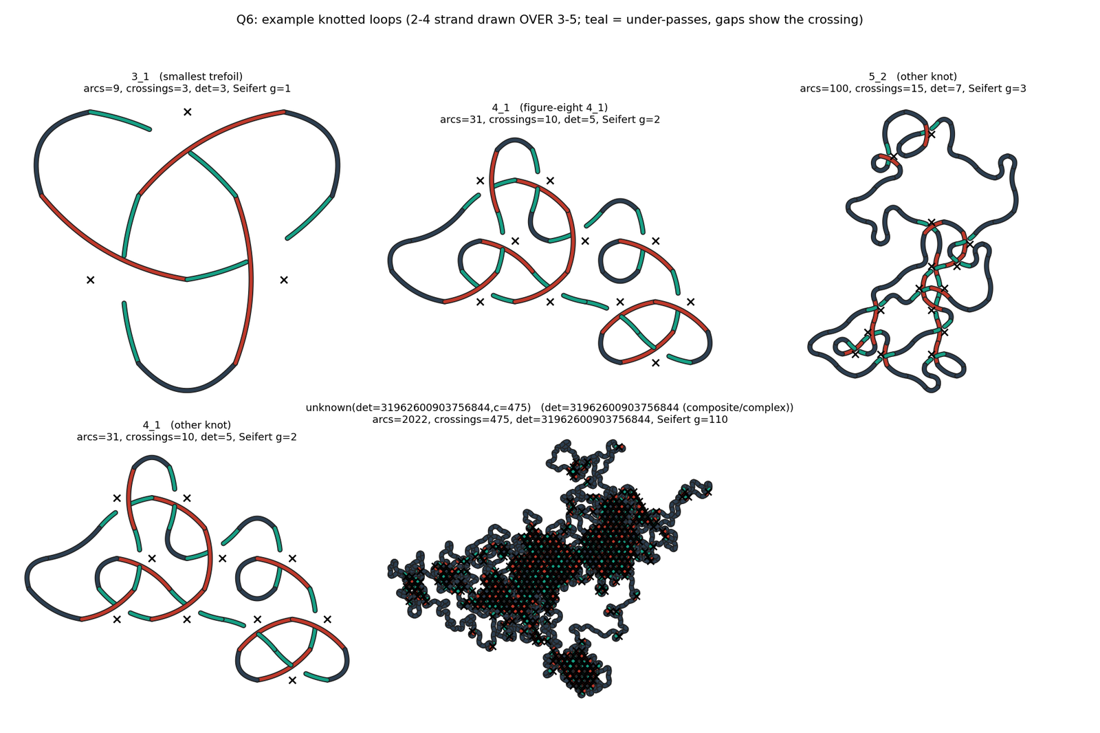
Consequence: every closed loop that visits a crossing tile simultaneously inherits an over/under label at that crossing. The loop, together with its crossing information, is precisely a knot diagram — a projection of a closed curve in 3-space onto the plane with explicit crossing data. The topology is not just an analogy; the invariants (determinant, Jones polynomial, genus) apply directly.
The smallest knotted loop is the trefoil 3₁, which requires a loop of at least 9 arcs spanning 6 tiles. The smallest loops (3 and 4 arcs, the triangle and rhombus) are always unknotted — they have no self-crossings. The first crossing that can contribute to a non-trivial knot appears at arc-length 6 (size-6 loops exist with 0 or 1 crossing), but the full trefoil requires 3 crossings simultaneously, which needs at least 9 arcs.
How common are knots?
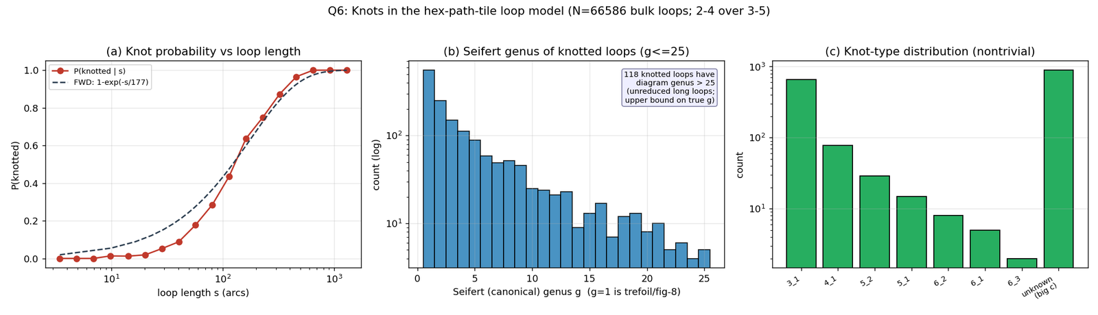
Most loops are short (the arc-length distribution is a power law s−2.11), so only a fraction are long enough to be knotted. But the knotting probability rises sharply with length: by s ≈ 177 arcs, half of all loops are knotted; by s ≈ 400 arcs, nine in ten are.
This is the Frisch-Wasserman-Delbruck (FWD) law:
The exponential form is proven for random polygons in 3-space; the measured decay constant N₀ ≈ 177 arcs is specific to this model. The complementary probability P(knotted | s) = 1 − e−s/177 is shown in the interactive widget below.
The small-knot census
Among knotted loops, the trefoil 3₁ is overwhelmingly dominant. The full zoo in order of frequency:
The trefoil's dominance is not surprising: at any fixed crossing number, the trefoil has the smallest arc-length, so it is encountered at the leading edge of the knotting transition. The fig-8 is amphichiral (mirror of itself), so it is found with both handedness conventions equally — in this model only left-handed trefoils appear, since the 2–4-over-3–5 rule fixes the chirality of all crossings.
Build a knot arc by arc
The widget below draws real loops extracted from the model as proper knot diagrams. Under-strands show the canonical gap at each crossing. Step through arcs one at a time to see how the knot structure assembles — and how the crossing handedness forces a non-trivial topology.
The trefoil in 9 arcs across 6 tiles is the global minimum: no smaller loop in this model can be non-trivially knotted. The figure-eight is the smallest amphichiral knot and requires 23 arcs — 2.5× as long. The 5₂ knot also needs 6 crossings but a different arrangement of 26 arcs.
56% of sharing-crossing loop pairs are linked
Two distinct loops can be linked: topologically entangled despite each being individually unknotted. Linking is measured by the linking number lk, a half-integer sum of the signs of the crossings shared between the two loops.
In the model, among all pairs of loops that share at least one crossing tile, 56% are linked (lk ≠ 0). The dominant example is the Hopf link (lk = ±1): a 4-arc rhombus loop and a 7-arc loop share a single crossing tile, and that one crossing gives lk = 1. The remaining 44% of crossing-sharing pairs have lk = 0 — shared crossings do not guarantee linking.
Higher linking numbers |lk| ≥ 2 are rare but present: they require multiple shared crossing tiles whose signs all agree, which is geometrically constrained on the hex lattice.
Slipknots: a knot hiding inside an unknot
Strictly, an open arc has trivial topology: it can always be isotoped to a straight line segment. "Is this open path knotted?" is ill-posed without a closure.
Our open paths, however, have both ends on the single outer boundary of the tiling. This gives a canonical exterior closure: join the two endpoints through the unbounded outer face without adding any new crossings. The closure is isotopy-unique and basepoint-invariant — it defines a genuine knot type for each open path.
Under the exterior closure:
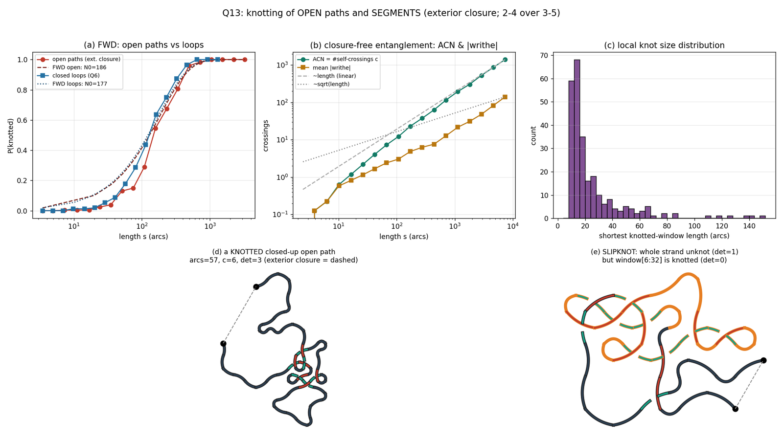
- 9.4% of open paths are knotted — 45% among those with ≥ 3 self-crossings.
- Same trefoil-dominated zoo as the closed loops.
- Same FWD law with decay constant N₀ ≈ 186 arcs (versus 177 for loops).
Slipknots: ~50% of long unknotted strands
A slipknot is an open path that is globally unknotted under exterior closure, yet contains a knotted sub-arc. The knotted region "slips out" past the free endpoints of the full strand — like a real slipknot knot that unties when you pull on both ends.
Scanning windows along long strands in the model: 89% of long strands contain a localized knotted sub-arc (median knot size ≈ 18 arcs), and ~50% of globally-unknotted long strands are slipknots. The paradox is genuine: the full strand is unknotted, but a sub-arc of it closes to a trefoil.
ACN ∝ length · |writhe| ∝ √length
Even without closure, open strands accumulate entanglement. Two distinct measures capture different aspects:
- Average crossing number (ACN) — the expected number of apparent crossings over all projection directions. ACN grows linearly with arc-length: ACN ≈ 0.034·s. This means a strand of 300 arcs has roughly 10 apparent crossings from any random viewpoint.
- Writhe — the signed sum of crossing signs (as a closed diagram). |writhe| grows as √(arc-length), the signature of a random walk accumulation. Each new crossing adds ±1 randomly, so the net writhe diffuses.
These two scalings — linear ACN vs. √-writhe — reflect two different facets of the geometry: ACN counts the total entanglement (which grows with the number of crossing pairs = quadratic in length, but averaged over projections gives linear scaling), while writhe is the net chirality, which random-walks.